
Warning: This is not so a small post, so grab a coffee and sit tight!
Functions in programming languages, Calculus in mathematics, observational data in Physics, experimental measurements in statistics, tables and attributes in RDBMS, all of them have one thing in common: 'variables'. So we deal with variables all the times. Variables come with data type and are either discrete or continuous in nature. In this article, you will learn how to classify variables between discrete and continuous. And what kind of challenges and opportunity this kind of classification can pose to you. You will find answer to following questions in the article:
What's the difference between a discrete and a continuous variable
Why you should care about the classification of variables
Once you have understood fundamental behind types of variables, in the next part of this post, we will discuss how we can manipulate and transform variables in the Tableau to make visualizations.
Blue and Green Pills
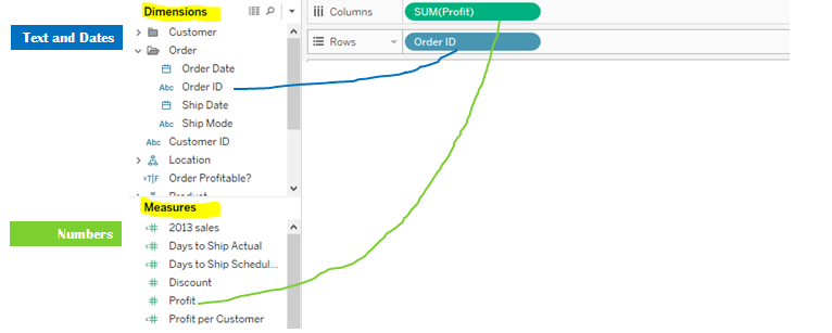
If you have worked in Tableau before, you'll notice, all of your data is divided between dimensions and measures. Dates, geographies, names, categories and non-numeric information goes into dimensions and anything numeric including latitude/longitude goes into measures. Here are a few observations which you must have noticed
Most of the dimensions are non-numeric and all of the measures are numeric
When you drag these elements into views to create visualization, the pill either turns blue or turns green
Blue pill means element is being treated as discrete variable, green pill means element is being treated as continuous variable
Most dimensions convert into blue pills, most measures convert into green pills
Looks like most dimensions are discreet, most measures are continuous
So good so far, but this is where things get confusing:
Variables can interchange between dimensions and measures (measures convert into dimension, dimensions convert into measure)
When you convert a textual dimension into measure, it converts from textual to distinct count and gives out a number (rather than the original text in the field) when dragged into view
Dates can be treated continuous as well discrete variable

Why does this happen? Why the behavior of a variable changes when its converted into other type of variable? Why dates can be both discrete and continuous? Why there is a blurry line between dimension-discreet and measures-continuous? Let's figure it out.
Discrete and Continuous
Google defines discrete as 'individually separate and distinct' and continuous as 'forming an unbroken whole; without interruption'
If you remember the Number Line from school maths, there is 0 at the center, move any right and you get positive numbers move any left and you get negative numbers. Integers jump from 0 to 1, 1 to 2, 2 to 3, -1 to -2, -10 to -11, they jump in multiples of 1, as in whole.. They don't land anywhere in between two integers. They are discrete on the number line. On the opposite, real numbers can take any possible value such as 1.1, 3.117, 9.99, 9.99999, 9.9999999999 or even irrational numbers like π = 3.14159265359..., √2 = 1.41421356…, e = 2.718281828... and can be marked on the Number Line. Subsequent natural numbers move swiftly on the line left and right unlike integers (that moved only in a certain gap of ±1). The break between two sequential natural numbers is ±1/∞ ≈ 0. So the gap between two consecutive natural numbers ≈ 0 or no break. And because of this no break, Natural Numbers are continuous on the Number Line.
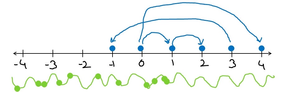
Wave and Particle: Continuous is everywhere on the number line you can think of, like a wave. Discrete can live only at particular places, like a particle!
Now we will come out of mathematics and take some example from the real world. Consider a variable you are interested in, let’s assume it is 'sales'. Now assign any random value to your variable that can think of. I assigned $1000. Now add or remove a very small quantity that you can. What's the new sales number? Mine is $999.96. Okay. Try it again. What's the new number? This time my guess is $1000.075. See, it is behaving like a continuous number on the Number Line. Sales is a continuous variable. So the essence is that if your variable can be broken down into many many small pieces and the meaning of variable doesn't change, it is a continuous variable.
Now let me ask you a different question. What is your shoe size? Mine is 43! Others will have like 42, 40, 46 and so on! Now notice something different? Shoe sizes are not taking any possible values but rather taking some certain values in the multiple of 1 cm. Now ask the same question with your feet size!
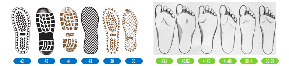
Shoe size is 43. But what is your feet size, measured with a scale? Try it now. Something tells me it's NOT exactly 43 :-)
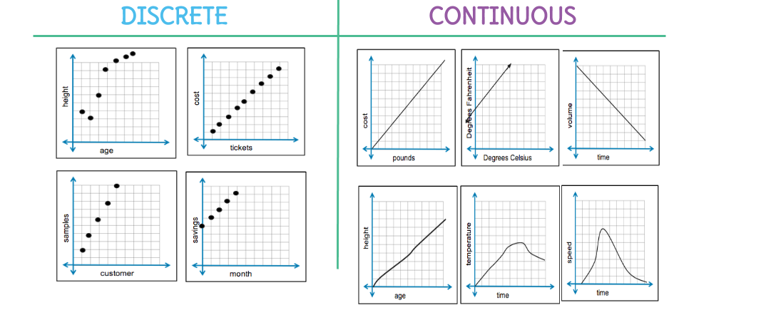
Types of Variable
Let me to show you a diagram, please!
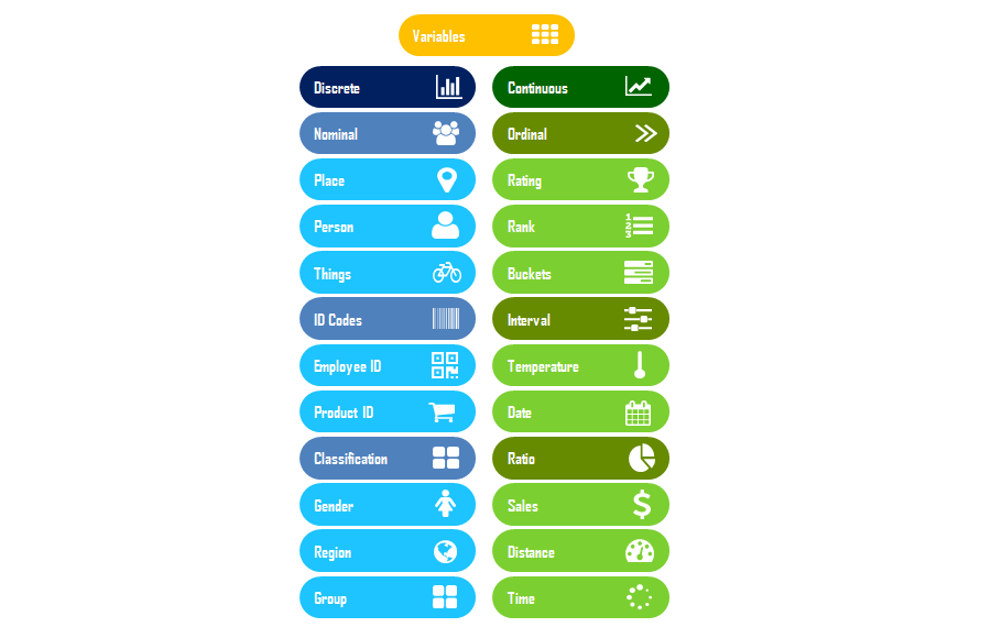
This is not a hard and fast classification, rather an indicative one that works well with most of my models. I would like to know how would you classify them!
Discrete Variables
Also known as qualitative variables tell you the attribute of the observation they are associated with. Further divided into following categories for your convenience
Nominal Variables : All nouns are nominal variables and come under discrete. That says, names of sales managers (people), geographies, countries, states and cities, even the addresses and zip codes (places), products and flowers (things) are discrete.
Categorical Variables: Property of something that cannot (or is not being) be expressed in numbers, categories of something are categorical variables. Region of a sales geography north, east, south, west, gender of a person male, female, income level an individual belongs to below poverty line, lower, middle, upper, upper-high, is some country developed yes, no. These are all categorical variables. Researchers sometimes like to express categorical variables using integers in their data like male as 0 and female as 1. But that doesn't make the variable from discrete to continuous. Because it is not the data-type of variable that expresses the type of it but the core property of the variable that is of interest itself.
Calendar Variables: I would like to talk about calendar variables separately. By calendar variables, I mean year, month, week, date, hour, minute and seconds. What is a date. Date is just a name given to any day so that we can identify it uniquely. Name? So date is a nominal variable which makes it discrete? Yeah! Now you see why calendar variables come as blue pill in Tableau! But also, dates are sorted in the certain order which makes them a ordinal continuous variables. Now you see why sometimes date converts into a green pill! More on this later.
Source: https://learnzillion.com/
Continuous Variables
Also known as quantitative variables tell you about magnitude of the observation they are associated with. Further divided into following categories for your convenience.
Ordinal Scale: In data analysis, you will come across a lot of values that are expressed in some order. Like rating of movies on IMDb from 1 to 10. Preference of some product from 1 to 5. Numbers in this kind of variables can tell you which ones come first and which ones later (or which are worst and which are best) but this is all you can do. You cannot say that movie with 8 rating is twice as much good as the one with 4. Or you cannot tell 'Like This Product A Lot' is how much strong preference than 'Product is OK'. In social research or market surveys, these are one of most common kind of variables and there are many methods to deal with the kind of limitation they pose to us. And even there are completely different practices in visualizing this kind of data. One important thing to remember in this kind of variables is that they do not have a 0 anchor point. As in 0 means 'nothing' of something but in ordinal variables, even 0 will have some meaning encoded into it , as in the product example, probably 0 will mean 'Least Like This Product'
You can only do comparison between two ordinal variables as such movie with 7 points > movie with 2 rating points but you cannot add them up i.e. you cannot say a movie with 5 rating point + a movie with 3 rating point = a movie with 8 rating points
Interval Scale: You can think of these variables as a range. Where you have some starting point and an ending points and their magnitude is taken by the distance between their starting and the ending point. Doesn't that sound like a Number Line where you measure the magnitude by taking interval between 0 and the point? Yeah, it does, except for the fact an interval variable doesn't have an absolute 0 point. Let me show you what do I mean.
The 0 point means absence of something at all the the origin point. Now the interval variable as such temperature also have the value 0 degree F. But does that mean absence of the temperature? Convert 0 degree F into a different unit and will have -18 degree C. That's not a zero! That's why they are known as interval variables. Because even though they have a zero point, it still doesn't mean absence of the quantity.
F x 1.8 + 32 = C
You can add (or subtract) two temperatures as such 10°F + 15°F = 25°F but you cannot divide or multiply them i.e. you cannot say 20°F = as twice hot as 10°F.
Interval variables are superior than ordinal variables because along with comparisons they also allow you to do addition and subtraction and help you do a better analysis.
Ratio Scale: When 0 means absence of the magnitude in the measurement, it is the ratio scale. Sales = $0 means no sales at all. Weight = 0 KM means no weight at all. These variables do not show different magnitude when measured in different units and will always show the same ratio hence, the name ratio scale.
As of today $1 = £0.82. Lets assume we have a product with $100 sales and $15 profit chance giving the profitability of 15%. Now if you change the unit from $ to £, sales becomes £82 and profit becomes £12.30. But the ratio still remains the same that is 15%.
We can do all sorts of basic mathematics operation on them meaningfully
$100 + $1,000 = $1,100
$5,000 = 2x $2,500 = 5x $1,000 = 1000x $5
Discrete & Continuous : Both at Same Time. Heck, Yeah!
If you have come this far, awesome! I hope you've enjoyed the post till now and still have some coffee left in your mug, let's continue...
You may have heard that an electron is a wave and particle both. Wave is continuous and particle is discrete. Some variables too behave the same way. The most obvious example is date. Sometimes we treat date as discrete and sometimes continuous. At first, this may seem confusing but it all depends upon how we use the variable or more specifically, what is the particular application in this certain case. If you think a little deeper, date also implies the time, the continuous flow of the stream of the moments. Time flows; in a continuous motion on the timeline and the flow of moments (tiny tiny tiny fractions of time) makes it a non-breaking stream.
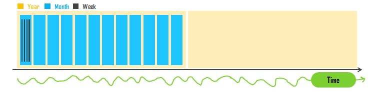
Continuous stream of time can be thought of made of small discrete time intervals such as years, months, weeks, days...
Now if you are thinking your time-series data as a stream that flew over a period of time, you can choose to keep your dates as continuous. You must have seen that in stock market trend visualizations. Also, it might be helpful to consider dates continuous variable when calculating forecast regression line for a time-series data where time is an independent variable on x-axis and the variable that we are trying to predict (a common use is to plot sales on a scatter-plot as dependent variable on y-axis.
A quanta is the minimum possible quantity of something that can possibly exist. As you've seen above, for counting things, the quanta is 1. The thing less than 1 is not the thing in itself, it's a broken thing and since broken thing is not the same as the thing, so things can only exist in the quanta of 1 and the possible quantity of something countable is n where n is non-negative integer.
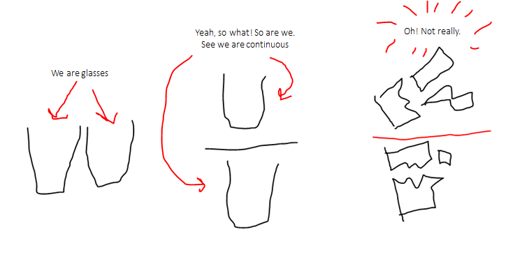
A broken glass is not a glass anymore, its a broken-glass!
There is a famous paradox in cartography known as Coastline paradox. The paradox says,'the coastline of a landmass does not have a well-defined length. This results from the fractal-like properties of coastlines.' Measurements of the coastline will very with the quanta that you use to measure the coastline. With the quanta = 100 km, coastline of Britain is 2,400 km whereas 3,400 km when quanta is reduced to 50 km. This error is introduced in the measurement because of the fractal structure of coastlines and we tried to measure coastline using a discreet scale, a quanta of 50 km resolution.
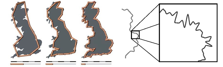
Source: https://en.wikipedia.org/wiki/Coastline_paradox
I sometimes wonder if the world (and the universe) is continuous or discrete! And the answer comes,'Both'. It depends in what context do you want observations to be measured and analyzed. A moving train has a continuous motion, but if you zoom your vision to atoms, you may think these are actually lots of atoms moving discretely. Again if you zoom further, and think atom as made of proton, neutrons with electrons circling all around in a probability cloud. You may again begin to wonder, that electrons around atoms are a fuzzy continuous clouds, so now you perception of tiny discrete atoms becomes the fuzzy uncertain cloud of tiny sub-particles and the perception once again changes from discrete to continuous.
So, I tell myself, zoom only till the certain level that is necessary for your data analysis, and I record motion of the train as a continuous variable. Another way to think of this is that how much accuracy you are willing to let go of in exchange for the ease of measurement that you are making.
Why is the Differentiation Important and How It Affects Data Analysis
Type of variable is important in the data analysis for three major reasons
It helps you define what kind of model you will require to process your data and what kind of algorithm you should run for analysis
It helps you decide how you will calculate your KPIs to summarize the results
It helps the software understand what kind of data it is, and different type of input variables will produce different type of output
It helps you decide which kind of visualizations can be produced with the data, and what is the right practice to communicate certain type of variables
Example 1: You have two continuous variables height and weight, and you want to establish relation between the both, you can use linear regression to model this relationship. However, if one of the variable is binary discrete (a discrete variable which has only two mutually exclusive possible outcomes) i.e. weight 'less than 60 kilos' and 'equals or more than 60 kilos', then the linear regression might not work as efficiently and you will need a different type of modeling probably a logistic regression. So different data types can make you choose a different data analysis method.
Example 2: In the data analysis, you often need to summarize the data. One of most used technique to summarize the data is to aggregate the data and show it in a small summary table or chart. There are many kind of aggregations that you can do like sum, average, standard deviation, median, counting, proportions and distinct counting of variables. You are limited to the kind of aggregation that you can do on the variable by the type of variable it is. If you can demographic data which has a variable gender, you obviously cannot add genders because male + female doesn't mean anything in the mathematics however, you can do the counting, and can tell that there are 20 million females and 19 million males in the population, you can do the proportioning and tell 51% population is female and 49% is male.
If you have customer names in sales data of some retail chain, you can distinct count customer codes and can number of unique customers that made a purchase at the store. If your variable is continuous, you can do almost all possible type of aggregation on the data like summing up sales, telling the sales growth from last quarter to this quarter, average age of population. The best kind of aggregations come from the combination of discrete and continuous variables and do the aggregation like average sales per customers where sales is the aggregation of a continuous variable, and unique count is the aggregation of a discrete variable and finally they are combined to calculate a new average that is average sales per customer.
Example 3: If variables make your data, KPIs make your analysis. Think of this: Interstellar: average movie score on IMDb 8.6, percent of critics rating positive on rotten tomato 71% as of 31/10/2016. Both of the KPIs show the rating of a movie however, the first one is measured as a continuous variable (rating from 1 to 10, in fact ordinal however, treated as continuous by IMDb) and takes average of ratings to show the movie performance however, the second one measures rating as binary discrete (liked or not liked) and calculates the ratings as proportion of critics who voted up for the movie. So the choice of variables makes an impact on how do you calculate your KPIs.
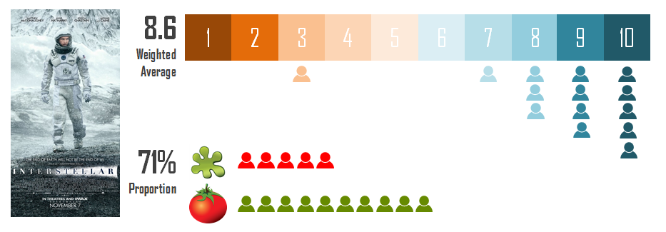
Numbers only for indicative purpose. Method described here is only for indicative purpose and differs from actual algorithm used by IMDb and Rotten Tomatoes.
Transformation of A Continuous Variable into Discrete
I am going to take the next example from economics. Income of any household is something researchers are always very interested in. Income is a ratio scale variable and comes under continuous variable category. However, since income is a sensitive personal information and individuals are reluctant or likely to lie when asked directly about their incomes. To overcome this problem, researchers rather ask for the range of their income such as $0 to 1,000, $1,000 to $2,500, $2,500 to $5,000, $5,000 or higher. This kind of bucketing not allows researchers to get better data quality, though there is some information loss in this process because you only know a certain income range in which the individual falls and not the specific income itself.
This kind of bucketing can be performed on existing continuous variables as well. You can assume you have sales of 20 stores which is a continuous variables. But you can convert sales into buckets and use the bucket as a discrete variable to tell how many stores fall within certain sales bucket. This kind of formation is very useful in certain scenarios and is often performed to simplify highly varying continuous scale variables into small number of classes where you can study each class separately or do the comparison among them.
Variable Reference Table : Few Examples
| Variable | Variable Type | Variable Scale |
|---|---|---|
| Family Income | Continuous | Ratio |
| Family Income Buckets | Discrete | Ordinal |
| Time Duration | Continuous | Ratio |
| Hour on the Clock | Discrete | Ordinal |
| Date* | Discrete | Nominal |
| Sales Figures | Continuous | Ratio |
| Country | Discrete | Nominal |
| Foot Size | Continuous | Ratio |
| Shoe Size | Continuous | Interval |
| Temperature | Continuous | Interval |
| Length | Continuous | Ratio |
| Product ID in Numbers | Discrete | Nominal |
| Gender | Discrete | Categorical |
| Gender as Binary 1/0 Coding | Discrete | Categorical |
| True/False | Discrete | Categorical |
| Phone Number | Discrete | Nominal |
| Area Code | Discrete | Nominal |
| Rating on 1 to 5 Scale | Continuous | Ordinal |
| Player Ranking | Continuous | Ordinal |
Next Steps
On purpose, I made it sound distinct that a variable is either discrete or continuous. While working with the data in the software in real life, few variables can be interchanged between discrete and continuous for a better analysis or visualization. The most obvious example of this is dates in Tableau where date is frequently treated as discrete as well continuous. We can call it variable transformation.
In the part II of this blog post, we are going to apply in Tableau what we have learned so far. We will use various variable transformation methods like creating bins, grouping, truncating dates, creating ranges, bucketing values and counting observations.
